Normalisation
Normalisation
Change Samples IDs by Sample names and save the table
Using the table furnished by Kontxi Martinez, Samples IDs are replaced by the experiment name in the read courn table. The experiment name follow the current pattern:
- Isolate_Replicate_Condition_Harvesting time
Import the corrected table
The corrected read count table is imported. Only value of the GREEN pair are kept. The homemade function LoadRawReadCounts() is used for this.
Normalisation
Read count are normalized using the ReadCountNormalisation() homemade function
- list of packages used
- better description of the global procédure
Low reads filtering
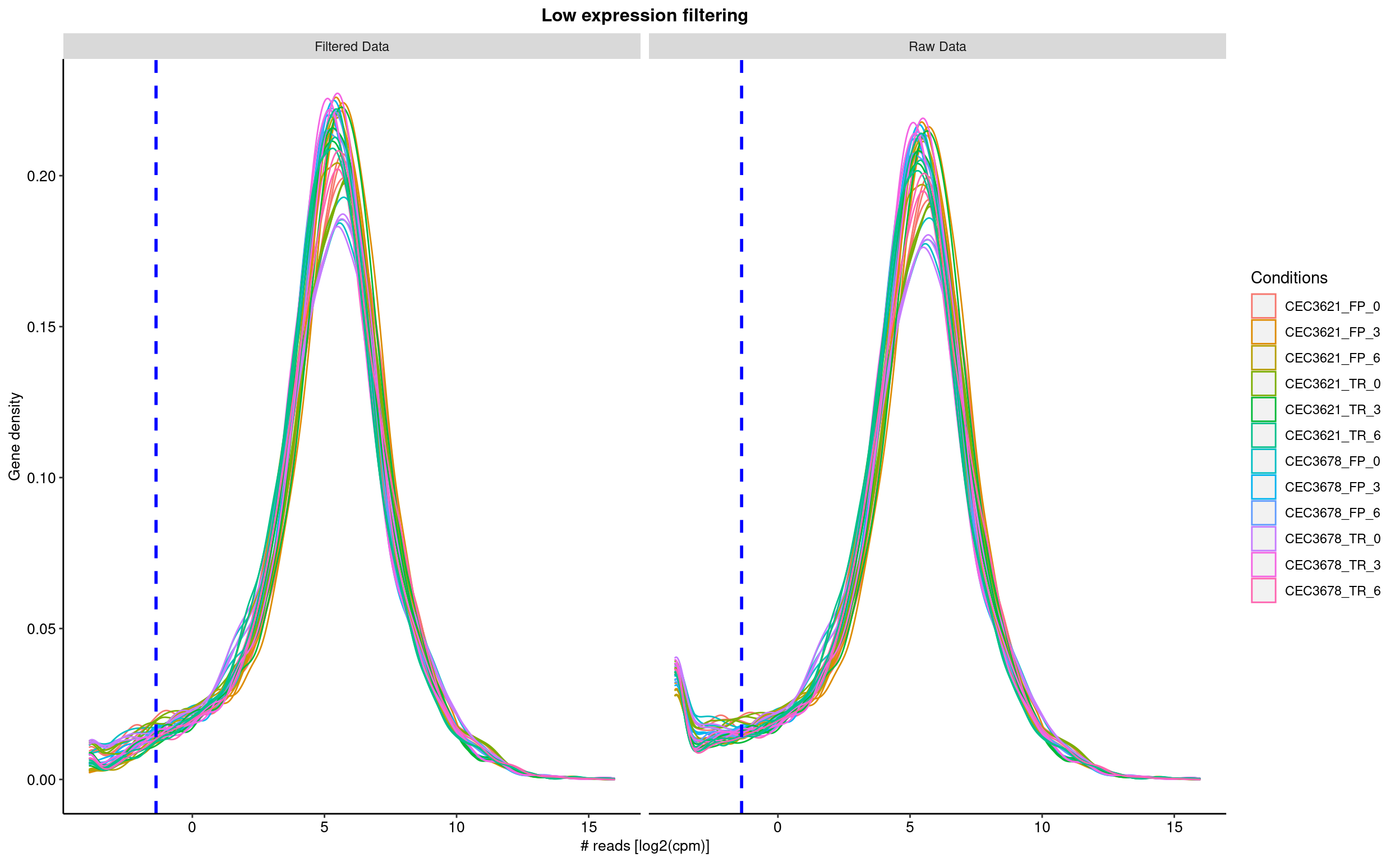
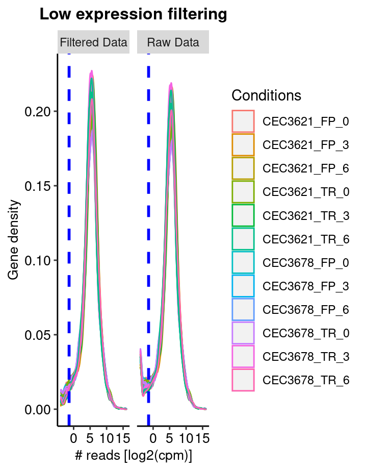
The first step consist in removing features, here genes, with no or low reads in all samples. The sequencing detection limit is estimated at 10. This means that genes with less than 10 reads in all samples are considered as not expressed (or expressed under the detection limit) and are thus removed from the analyis. Here, 0 genes have been rejected. The filtering is based on the the filterByExpr from the edgeR packgage. The figure shows the density of gene read counts. Note the vertical line indicating the threshold used to sort out none expressed genes.
Sequencing depth
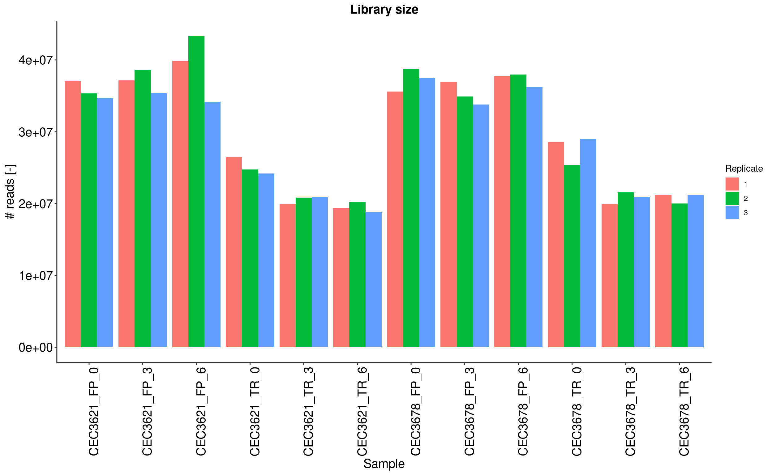
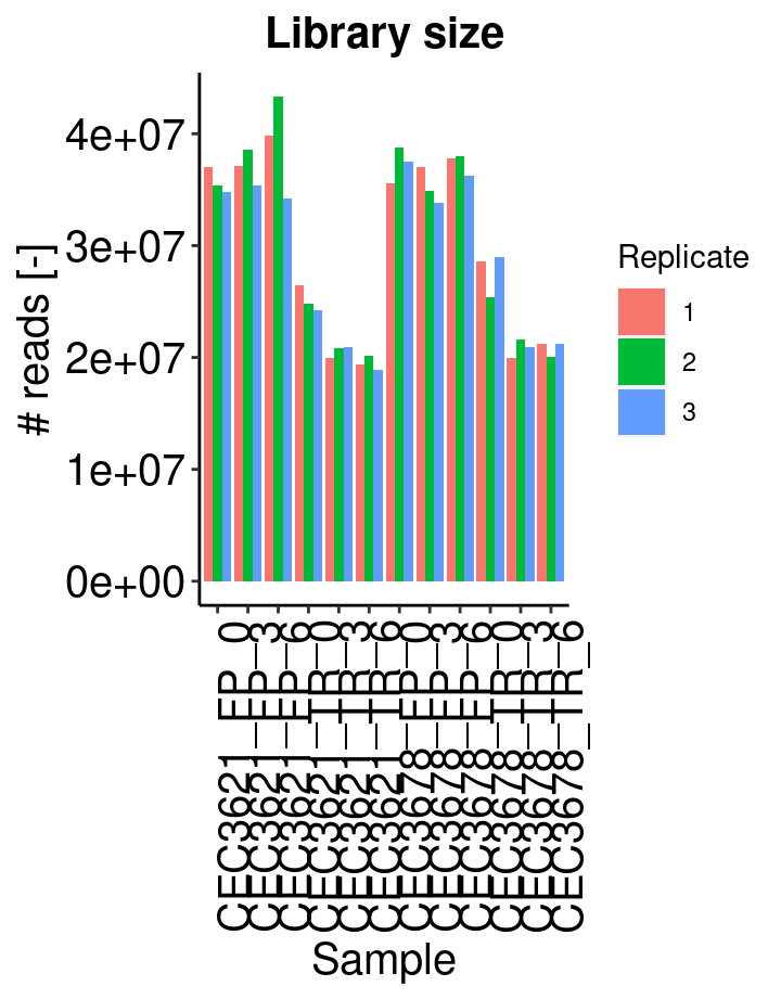
Barplot shows the whole number of read counts for each sample. Reads which are not associated to an annotated gene, are not considered in the calculation.
A filtering is also applied to identify and remove genes with less than 10 reads (see the Low read filtering tab). Reads associated to these filtered out genes are rejected.
TMM based data correction
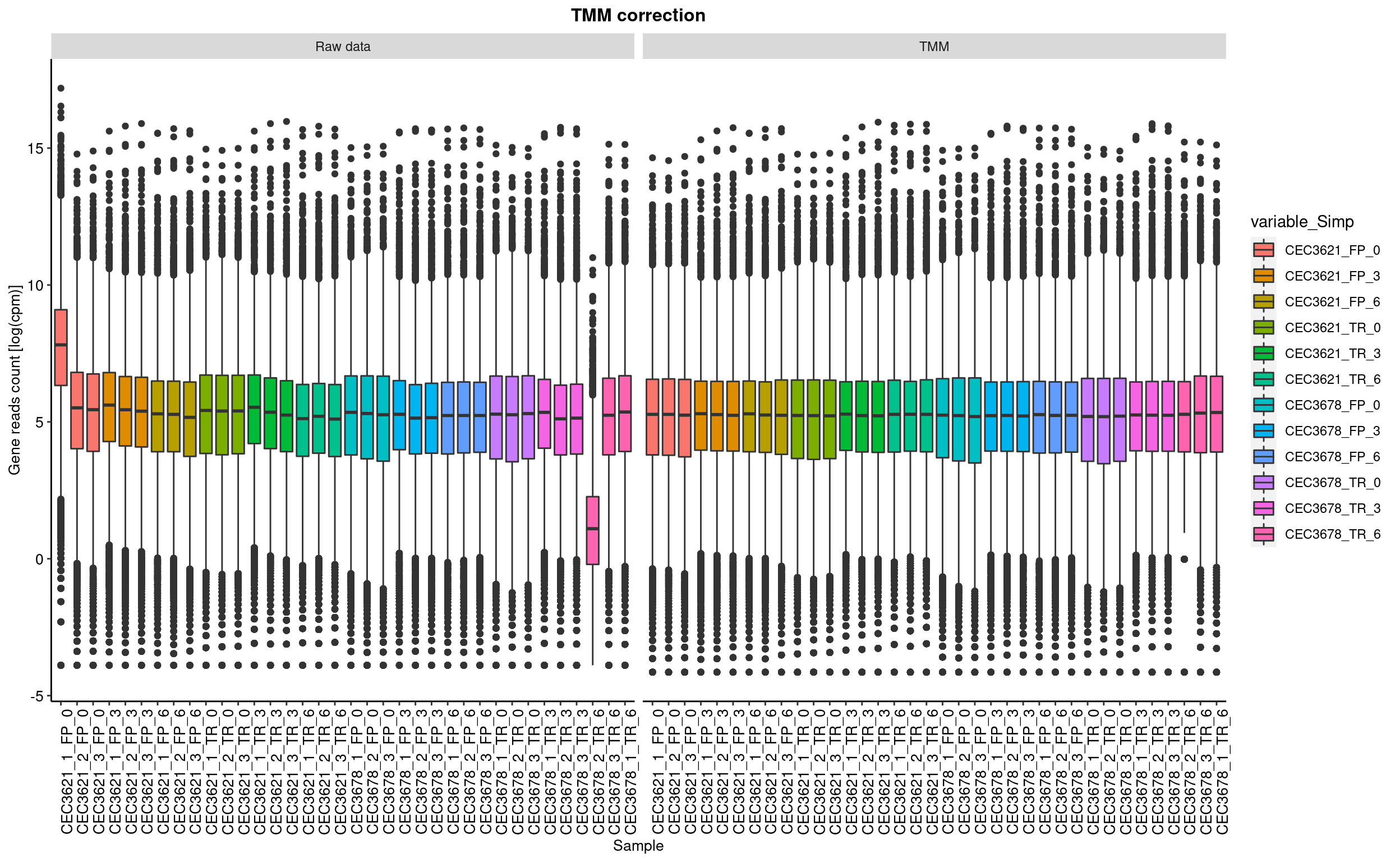
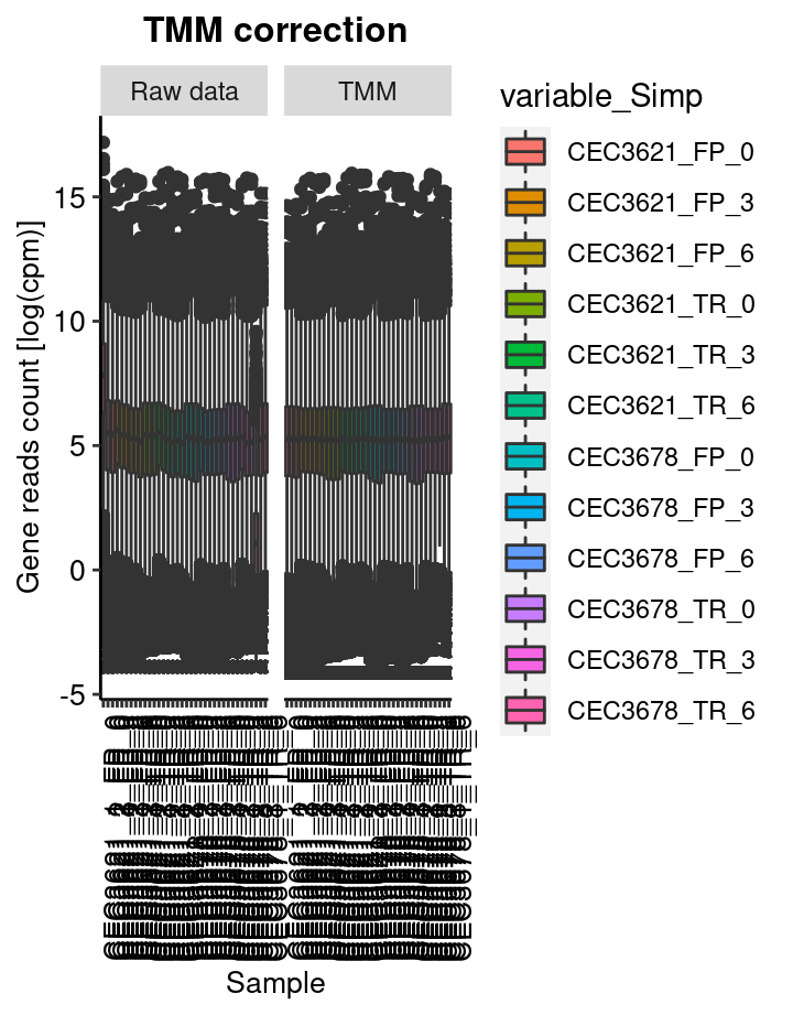
This step consist in removing the compositions bias using the TMM (Trimed mean of M-value) Robinson and Oshlack 2010. In short, samples with different library size cannot be compared with each other. The process consist in normalise the read count such like each sample have artificially the same total number of reads.
The calcNormFactors from the edgeR package has been used to perform this process.
boxplot represent the distribution of genes log2(cpm). cpm are count per milion of read.
Voom transform of read counts
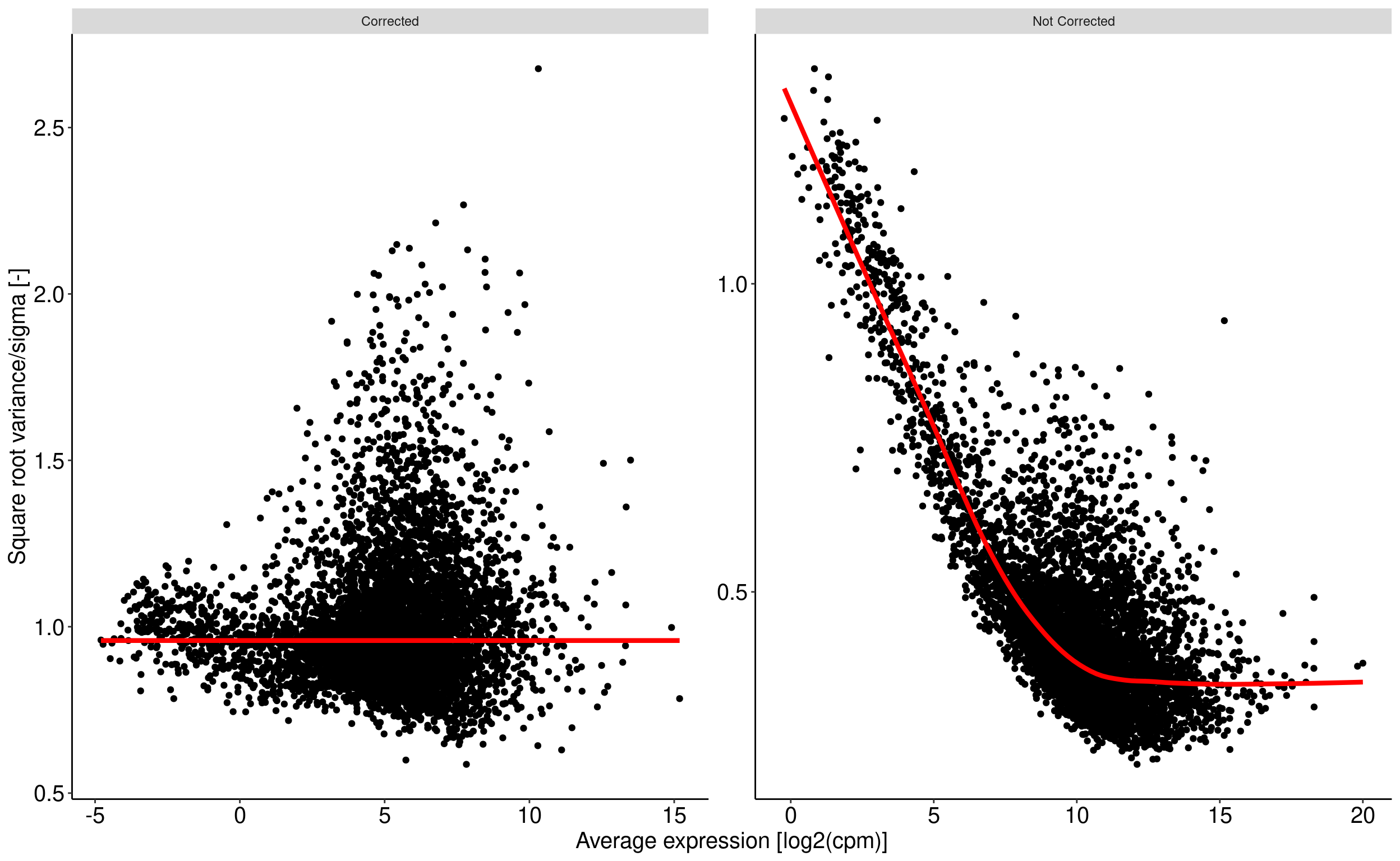
Voom transform of counts : removing heteroscedascity from count data
The basic principle is to remove a bias related to the relationship between gene expression variance and gene expression mean. The more condition/replicate we have the better it is. voom aim at prepare the data for a further linear fit see chapter 6.2 of RNA-seq analysis is easy as 1-2-3 with limma, Glimma and edgeR. This operation is performed using the voom function from the limma package.
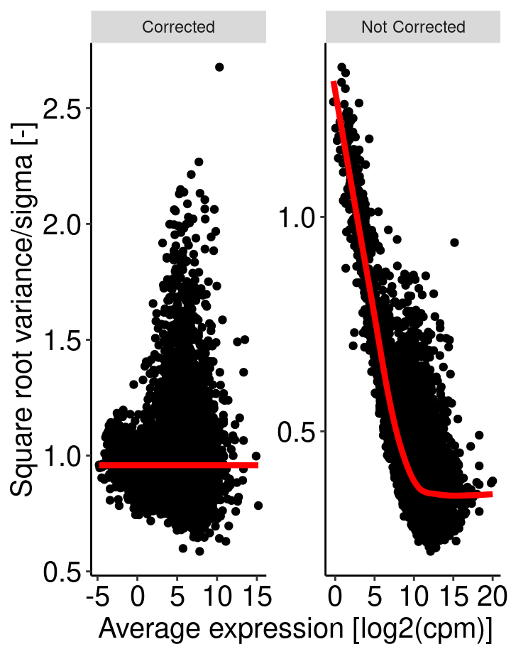
For a given data set with multiple samples, it is expected the average read count associated to a genes should not depend on its variance. More simply, the variability among samples should be similar for every genes and not depends on their average expression level. For RNAseq data, this relationship between variability and expression is unfortunaltely true (figure right). Lower will be global number of reads associated to a gene, higher will be the variability among samples. This may have an impact on p-value when comparing the expression of gene between two samples.
Voom transform attempt to correct for this bias. From the comparison of the standard deviation against the average read count of each gene, a model is built (right panel, red line) and used to correct read counts value (left panel).
Batch effect correction: PCA
This step might not be essential since all samples are from the same batch. This can be interesting if sequencing files come from different runs or lanes. We will use the SVA package to infer the batch effects. Very quickly sva estimate the number of covariate (surrogate variable) and then adjust value to remove the noise associated to such covariate. Then adjust for the batch effects using Surrogate variables. Here the strategy consist in let the algorithm estimate the potential batch variables rather than feeding it with known source of batch effect.
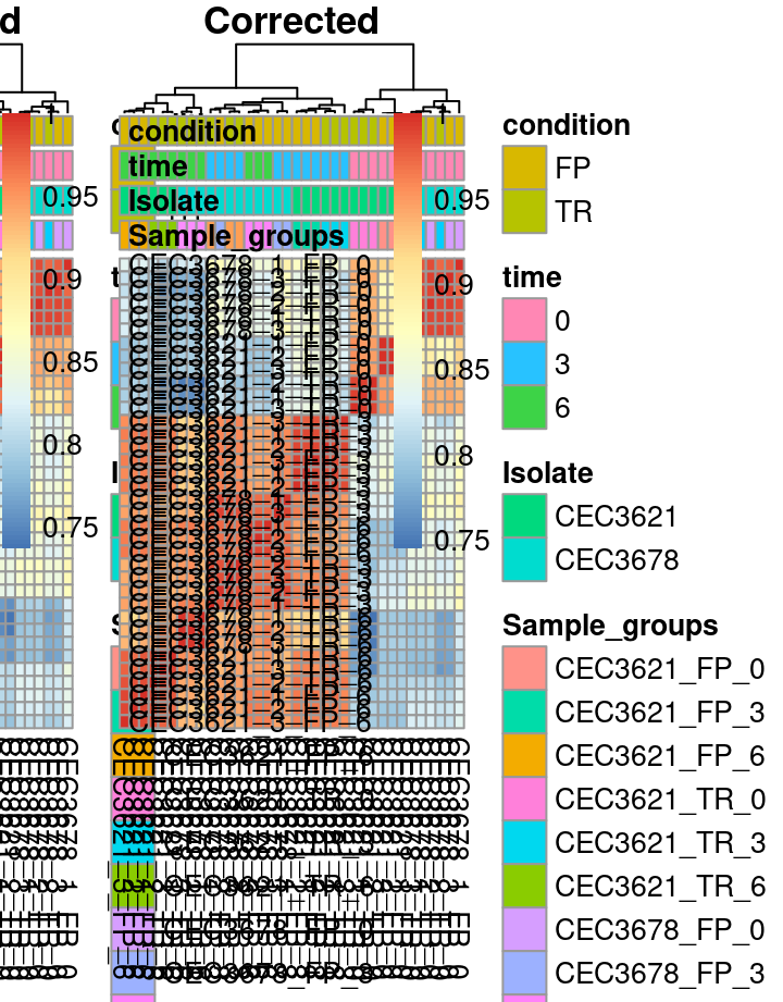
Different visualisation can be used to observe the correction of the batch effect. The first is the PCA. PCA plot is a scatter where each dot is a sample. Ideally, all replicates from a given condition should appears close from each other, indicating a good reproducibility. Our strategy based on the estimation of variables inducing noise may reduced the distance between replicates on the PCA plot.
